ML Application to Predicting Stock Prices using ARIMA

Install the required libraries

%%capture
!pip install yfinance
!pip install pmdarima

%%capture
import yfinance as yf
import pandas as pd
import numpy as np
from statsmodels.tsa.arima.model import ARIMA
from sklearn.metrics import mean_squared_error
import pmdarima as pm
from datetime import datetime

# Define the company's stock symbol
stock_symbol = "NKE"

# Import the data of last five years
start_date = "2018-04-21"
end_date = "2023-04-20"

# Save the imported data into a data frame
data = yf.download(stock_symbol, start=start_date, end=end_date)

# Print the data
data.head()

[*********************100%%**********************]  1 of 1 completed

	Open	High	Low	Close	Adj Close	Volume
Date
2018-04-23	66.000000	67.029999	65.949997	66.879997	63.032211	6338400
2018-04-24	67.309998	67.510002	66.720001	66.970001	63.117039	8176100
2018-04-25	66.839996	67.000000	66.250000	66.669998	62.834290	5188900
2018-04-26	66.779999	68.290001	66.639999	68.050003	64.134903	5355200
2018-04-27	68.470001	70.000000	68.449997	69.559998	65.558022	7814900

# Extracting the adjusted closing price data from the stock data and converting it into a pandas series
stock_price = data['Adj Close']
stock_price_series = pd.Series(stock_price)

print(stock_price_series)

Date
2018-04-23     63.032211
2018-04-24     63.117039
2018-04-25     62.834290
2018-04-26     64.134903
2018-04-27     65.558022
                 ...    
2023-04-13    125.172531
2023-04-14    124.697304
2023-04-17    124.934914
2023-04-18    124.954720
2023-04-19    124.420090
Name: Adj Close, Length: 1257, dtype: float64

# Split the data into training and testing sets
from sklearn.model_selection import train_test_split
train_data, test_data = train_test_split(stock_price_series, test_size=0.2, shuffle=False)

# Build the model
model = pm.auto_arima(train_data, seasonal=False, suppress_warnings=True)

# Train the model on the training data
model.fit(train_data)

ARIMA(order=(2, 1, 2), scoring_args={}, suppress_warnings=True)

%%capture
# Predict/ Validate the model on test data
predictions = model.predict(n_periods=len(test_data))

# Check the accuracy of the model. Here we are calculating Root Mean Square Error to check accuracy.
rmse = np.sqrt(mean_squared_error(test_data, predictions))
print('Root Mean Squared Error, RMSE:', rmse)

Root Mean Squared Error, RMSE: 29.22101157293209

Plot the actual and predicted values on a graph

import plotly.graph_objects as go
import plotly.offline as pyo

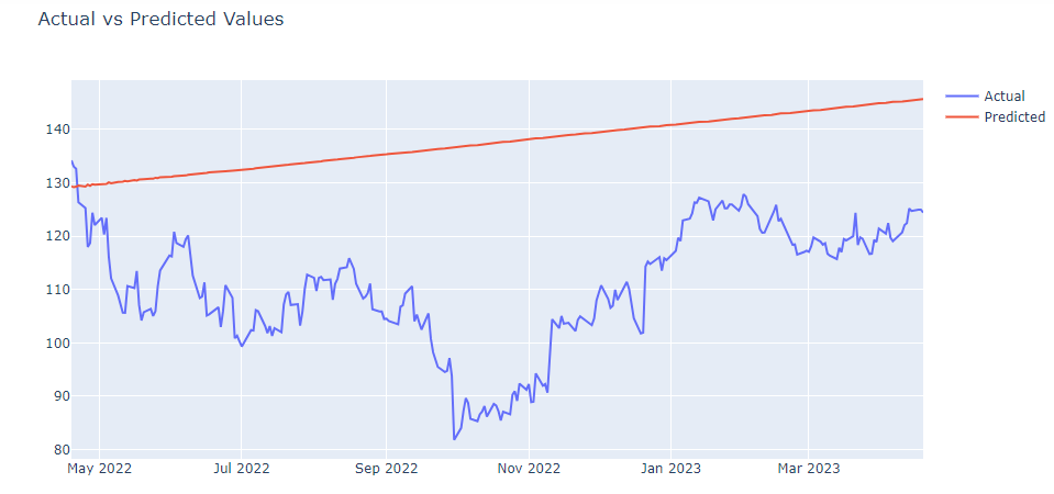
# create traces for actual and predicted values
actual_trace = go.Scatter(x=test_data.index, y=test_data.values, name='Actual')
predicted_trace = go.Scatter(x=test_data.index, y=predictions, name='Predicted')

# combine the traces into a data list
data = [actual_trace, predicted_trace]

# create the layout
layout = go.Layout(title='Actual vs Predicted Values')

# create the figure
fig = go.Figure(data=data, layout=layout)

# show the figure
pyo.iplot(fig)

# Predict a single value from a given date input
future_date = datetime(2022, 1, 2)
future_data = model.predict(n_periods=1, exogenous=None, return_conf_int=False, alpha=0.05, start=None)
print('Predicted Adjusted Closing Price for {}: '.format(future_date), future_data)

Predicted Adjusted Closing Price for 2022-01-02 00:00:00:  1005    129.307367
dtype: float64

# Print the predicted value for the input date
print('The predicted value for {} is: {}'.format(future_date, future_data))

The predicted value for 2022-01-02 00:00:00 is: 1005    129.307367
dtype: float64